
Probability is the mathematical language of uncertainty. The mechanics are simple: a number between 0 and 1 expressing how likely something is to happen. The trouble is that human intuition is famously unreliable at probability, especially when events combine or when conditional information arrives. A handful of foundational rules clears up most of the confusion.
Key Takeaways
- Probability is always a number between 0 (impossible) and 1 (certain), often expressed as a percentage.
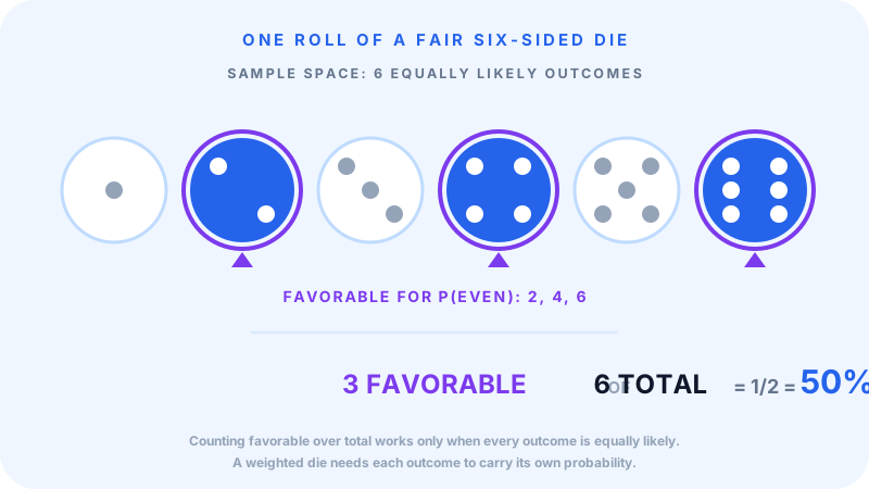
- P(event) = favorable outcomes / total outcomes for equally likely outcomes.
- Independent events: probabilities multiply. P(A and B) = P(A) × P(B).
- Dependent events: require conditional probability. P(A and B) = P(A) × P(B given A).
- Expected value = Σ (outcome × probability). The long-run average over many trials.
The Three Basic Rules
Rule 1: Probability is between 0 and 1. P(event) = 0 means the event cannot happen. P(event) = 1 means it certainly will. Everything else is somewhere between.
Rule 2: All possible outcomes sum to 1. P(rain) + P(no rain) = 1. P(heads) + P(tails) = 1.
Rule 3: Complement rule. P(not A) = 1 − P(A). If the probability of rain is 0.3, the probability of no rain is 0.7.
These three rules govern everything that follows.
The Basic Formula
For events where each outcome is equally likely:
P(event) = number of favorable outcomes / total number of possible outcomes
- Rolling a 4 on a fair 6-sided die: 1/6 ≈ 16.7%
- Drawing a heart from a standard deck: 13/52 = 1/4 = 25%
- Picking a vowel from "PROBABILITY": 4/11 ≈ 36.4%
If outcomes are not equally likely, you need to know each outcome's specific probability and sum them.
Independent vs Dependent Events
Independent events: the outcome of one event doesn't affect the other.
Probability of both happening: P(A and B) = P(A) × P(B)
- Flipping heads twice in a row: 1/2 × 1/2 = 1/4
- Rolling a 6 and then a 6 again: 1/6 × 1/6 = 1/36
- Drawing a king with replacement, then another king: 4/52 × 4/52 = 16/2704
Dependent events: the outcome of one event changes the probability of the next.
P(A and B) = P(A) × P(B given A)
- Drawing two kings without replacement: 4/52 × 3/51 = 12/2652 ≈ 0.45%
- Selecting two specific people in order from a group of 10: 1/10 × 1/9
The "without replacement" framing is the most common source of dependence in problems.
Mutually Exclusive vs Overlapping Events
Mutually exclusive: two events cannot happen at the same time.
P(A or B) = P(A) + P(B)
- Drawing a king or a queen (single draw): 4/52 + 4/52 = 8/52
Mutually exclusive is not the same as independent, and the two get confused constantly. Independent events can happen together; that is exactly what P(A and B) = P(A) × P(B) describes. Mutually exclusive events cannot happen together at all, so P(A and B) = 0. It follows that two mutually exclusive events with non-zero probabilities are always dependent: learning that one occurred tells you with certainty that the other did not.
Overlapping events: they share outcomes.
P(A or B) = P(A) + P(B) − P(A and B)
- Drawing a king or a heart: 4/52 + 13/52 − 1/52 = 16/52 (one king of hearts overlaps).
The subtraction prevents double-counting.
Conditional Probability
Conditional probability is the probability of A given that B has already happened:
P(A | B) = P(A and B) / P(B)
Example: In a population, 40% of people own a dog, 30% own a cat, and 12% own both. The probability that a dog owner also owns a cat:
P(cat | dog) = P(cat and dog) / P(dog) = 0.12 / 0.40 = 30%
Conditional probability is the engine behind medical test interpretation, recommendation algorithms, and Bayesian reasoning.
Bayes' Theorem (Briefly)
Bayes' theorem flips conditional probability:
P(A | B) = [P(B | A) × P(A)] / P(B)
It is the math behind updating beliefs given new evidence. A classic application: medical testing.
Example: A disease affects 1% of the population. A test is 95% accurate (true positive) and has a 5% false positive rate. If you test positive, what's the probability you actually have the disease?
P(disease | positive) = (0.95 × 0.01) / [(0.95 × 0.01) + (0.05 × 0.99)] ≈ 16.1%
This counterintuitive result (a 95% accurate test giving only 16% real-positive rate) is one of the most important applications of Bayes' theorem in everyday reasoning. Rare events stay rare even after positive evidence; you need much stronger tests to flip the conclusion.
Expected Value
Expected value is the long-run average outcome of a probabilistic event:
E = Σ (outcome × probability)
Example: A lottery costs $2 to play. Possible outcomes:
- 1/1000 chance of $1,500
- 1/100 chance of $20
- Otherwise nothing
E = (1/1000 × $1,500) + (1/100 × $20) + (989/1000 × $0) E = $1.50 + $0.20 + $0 E = $1.70
You pay $2 to play, expected return is $1.70: a net expected loss of $0.30 per ticket. Every commercial lottery has negative expected value; that's why they're profitable for the operator.
Expected value is the foundation of insurance pricing, gambling math, investment analysis, and decision theory under uncertainty.
Worked Example: Five-Card Poker
What is the probability of being dealt a pair (exactly two of a kind) in a 5-card hand from a standard deck?
Total possible 5-card hands: C(52, 5) = 2,598,960.
A "one pair" hand: choose the rank for the pair (13 options), choose 2 of 4 suits for that rank (6 ways), choose 3 different ranks for the remaining cards (C(12, 3) = 220 ways), and choose a suit for each of those (4 × 4 × 4 = 64 ways).
Hands with one pair: 13 × 6 × 220 × 64 = 1,098,240.
P(one pair) = 1,098,240 / 2,598,960 ≈ 42.3%
Poker probability is where combinatorics and probability meet most cleanly, and where intuition fails most often.
Common Mistakes
Gambler's fallacy. Independent events don't "remember" past outcomes. After 7 reds on roulette, the next spin pays black with exactly the same chance as before: 18 of 37 pockets on a European wheel (about 48.6%) or 18 of 38 on an American wheel (about 47.4%). It was never a true 50/50 because of the green zero, and the run of reds does not improve it. The wheel does not "owe" you a black.
Confusing independent and dependent. Drawing two aces with replacement is 4/52 × 4/52. Drawing two aces without replacement is 4/52 × 3/51, because the first card leaves the deck. Applying the independent formula to a dependent situation is one of the most common errors in probability work.
Ignoring base rates. A 95% accurate test for a rare disease still produces mostly false positives because the disease is rare.
Adding non-mutually-exclusive probabilities. P(A or B) is not P(A) + P(B) if they can both happen.
Treating low-probability events as impossible. A 1-in-10,000 event will happen, on average, once in 10,000 trials. Not never.
Confusing probability and odds. Probability of 1/4 = 0.25 = 25%. Odds of 1:3 = same probability, different notation.
Practical Scenarios
Scenario 1: Backup strategy. A disk has a 1% chance of failure in a year. Two independent disks: P(both fail) = 0.01 × 0.01 = 0.0001 (0.01%). Redundancy makes catastrophic failure much rarer.
Scenario 2: Vaccine effectiveness. A 90% effective vaccine doesn't mean 10% of vaccinated people get sick. It means the vaccinated are 90% less likely to catch the illness than the unvaccinated, a relative reduction, not an absolute one.
Scenario 3: Coupon strategy. A campaign distributes 100,000 coupons with a 4% redemption rate. Expected redemptions: 4,000. Standard deviation of binomial: √(100,000 × 0.04 × 0.96) ≈ 62. So redemptions land between roughly 3,876 and 4,124 (±2 SDs) about 95% of the time, which is a strong expectation rather than a guarantee.
Scenario 4: Defensive driving. A driver has a 1% chance of an accident in any given year. Over 30 years, P(no accident) = 0.99^30 ≈ 0.74. P(at least one accident) ≈ 26%. Small annual probabilities compound to substantial lifetime probabilities.
FAQ
What's the difference between probability and odds? Probability is favorable / total (e.g., 1/4). Odds is favorable : unfavorable (e.g., 1 : 3 for the same situation). Both describe the same likelihood with different notation.
What is independent probability? Two events are independent if the outcome of one does not affect the probability of the other. Coin flips and dice rolls are typical independent events.
How do you calculate the probability of multiple events? Multiply if independent (P(A and B) = P(A) × P(B)). For dependent events, use conditional probability. For "or" calculations, add and subtract the overlap.
What is expected value? The long-run average outcome of a probabilistic process: Σ(outcome × probability). It is the right summary number for decisions made repeatedly under uncertainty.
Why does the gambler's fallacy not work? Independent events don't depend on prior outcomes. A coin has no memory of previous flips. Streaks happen by chance and don't change future probabilities.
What is a fair coin? A coin where P(heads) = P(tails) = 0.5. A physical coin that is flipped and caught is very close to fair, and the residual bias is negligible for everyday purposes. Spinning a coin on a table is a different case: uneven weight around the rim can make spins measurably biased toward one face.
Can probability be greater than 1? No. Probability is bounded between 0 and 1. Numbers above 1 occur in odds, likelihoods (in some statistical contexts), or simple error.
Related Tools
The Probability Calculator handles single and combined events. For physical-randomness intuition, try Coin Flip, Dice Roller, and Random Number Generator.
Related Articles
Final Thoughts
Probability is one of the most powerful and least intuitive branches of math. The rules are short; the applications are everywhere. Master the basics (independence, conditional probability, complement rule, expected value) and most everyday probability questions become straightforward. The gambler's fallacy, the false-positive paradox, and the "100% chance" misuses of language all dissolve once you can sketch the math on a napkin.