
A score of 82 means nothing on its own. If the class average was 95, it is poor. If the average was 61, it is strong. The number did not change; the context did.
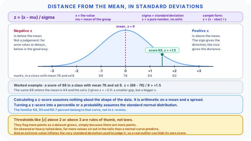
A z-score supplies that context in a fixed unit. It answers one question: how far is this value from the mean, measured in standard deviations?
That is all a z-score is. It is a rescaling, not a verdict, and most misuse comes from treating the result as more than a rescaling.
Key Takeaways
- z = (x − μ) / σ. Subtract the mean, divide by the standard deviation.
- z = 0 means the value is exactly at the mean. Positive is above, negative is below.
- The magnitude is the distance in standard deviations. z = 2.5 sits two and a half standard deviations from the mean.
- Calculating a z-score does not assume normality. Normality enters only when you convert a z-score into a probability or a percentile.
- Thresholds such as |z| > 2 or |z| > 3 are rules of thumb, not laws, and they behave badly on skewed or heavy-tailed data.
- Standardising makes different scales comparable only when the two reference groups are themselves comparable.
The Formula And Its Parts
z = (x − μ) / σ
| Symbol | Name | What it is |
|---|---|---|
| x | The value | The single observation you are placing in context |
| μ | Mean (mu) | The average of the population you are comparing against |
| σ | Standard deviation (sigma) | The typical spread of that population around its mean |
| z | Z-score | The distance from the mean, counted in standard deviations |
The numerator, x − μ, is the raw deviation in the original units: pounds, milliseconds, marks. Dividing by σ converts that deviation into a number of standard deviations, which is a pure number with no units at all.
That cancellation is the whole trick. It is also why z-scores are called standardised values: whatever you started with, you end up on the same scale. In the standard normal distribution, the mean is 0 and the standard deviation is 1, and a z-score is exactly a value expressed on that scale (NIST/SEMATECH).
Use the Z-Score Calculator when you have a value, a mean and a standard deviation. The Standard Deviation Calculator finds σ or s from a dataset, and the Average Calculator finds the mean.
Population Or Sample: Which Symbols You Are Using
The formula above uses population parameters: μ and σ, the true mean and standard deviation of the whole group you care about.
In practice you usually have a sample, and the standardised value is written with sample statistics:
z = (x − x̄) / s
where x̄ is the sample mean and s is the sample standard deviation.
Two differences worth keeping straight:
They are calculated slightly differently. The population standard deviation divides the summed squared deviations by N. The sample standard deviation divides by n − 1, a correction that makes s a better estimate of σ from limited data. Most calculators and spreadsheets offer both; picking the wrong one on a small sample changes the answer noticeably, and on a large one barely at all.
They carry different certainty. A z computed from μ and σ is an exact statement about position. A z computed from x̄ and s is an estimate, because both the centre and the spread were themselves estimated from the same limited data. On a sample of ten, s is unstable, and a z-score built on it is no firmer than the s underneath it.
Statistical texts reserve a separate symbol, t, for inference when σ is unknown and the sample is small. That is a hypothesis-testing matter rather than a descriptive one, but it exists for exactly this reason: standardising by an estimated spread is not the same as standardising by a known one.
Reading The Result
z = 0. The value is exactly the mean.
Positive z. Above the mean. z = 1 is one standard deviation above, z = 1.5 is one and a half.
Negative z. Below the mean. z = −2 is two standard deviations below. Negative is not a judgement: for delivery time or error rate, below average is the good direction.
The magnitude is distance. |z| = 0.3 is thoroughly ordinary. |z| = 3 is far out on the scale of that dataset's own variability.
What a z-score never tells you is whether a value is good. It reports position relative to one reference group. The sign gives direction, the size gives distance, and the domain gives meaning.
Worked Example
A student scores 88. The class mean is 76, and the standard deviation is 8.
z = (88 − 76) / 8 = 12 / 8 = 1.5
The score is 1.5 standard deviations above the class mean.
Now the same 88 in a different class, where the mean is 84 and the standard deviation is 2:
z = (88 − 84) / 2 = 4 / 2 = 2.0
The raw score is identical and the gap from the mean is smaller, four marks rather than twelve, yet the z-score is larger. In a tightly clustered class, four marks is a bigger departure from typical than twelve marks is in a widely spread one.
This is the point of the standardisation. Spread is the ruler, and different groups have different rulers.
Going the other way. Rearranging gives x = μ + zσ. In the first class, a z of −1.25 corresponds to 76 + (−1.25 × 8) = 66 marks. Useful when a threshold is specified in standard deviations and you need it in real units.
Comparing Values On Different Scales
A z-score is the standard way to compare measurements that have nothing in common as raw numbers.
A candidate scores 620 on a test with mean 500 and standard deviation 100, and 28 on a different test with mean 21 and standard deviation 5.
- First test: (620 − 500) / 100 = +1.2
- Second test: (28 − 21) / 5 = +1.4
The second result is the stronger of the two relative to its own cohort, which no comparison of 620 against 28 could have told you.
The caveat is the one that gets skipped: standardising removes the units, not the differences between reference groups. Two z-scores are comparable only if the groups behind them are. A z of +1.4 among self-selected applicants is not the same achievement as a z of +1.4 across everyone, even though the arithmetic is identical. Comparing a child's height z-score against an adult reference produces a number and no information. The reference group is part of the statistic, even though it does not appear in the formula.
Where Normality Does And Does Not Matter
This is the distinction that matters most, and it is regularly collapsed.
Calculating a z-score does not require a normal distribution. Any dataset with a mean and a standard deviation can be standardised. Subtracting the mean and dividing by the standard deviation is arithmetic; it makes no assumption about the shape of the distribution. Whatever the shape, the standardised values always have a mean of 0 and a standard deviation of 1.
Interpreting a z-score as a probability or a percentile does require an assumption about shape. The moment you say "z = 2 means roughly the 98th percentile" or "that is a 1-in-40 event", you have stopped describing and started modelling, and the model is the standard normal distribution. The percentages attached to z-scores, the familiar figures of about 68% within one standard deviation, about 95% within two and about 99.7% within three, are properties of the normal distribution, not of z-scores.
So a z-score computed on strongly skewed data is a perfectly valid description of position. It is the percentile claim laid on top of it that fails.
One distribution-free result holds regardless of shape: Chebyshev's inequality guarantees that at least 1 − 1/k² of any distribution lies within k standard deviations of the mean. That is at least 75% within two and at least 88.9% within three, for any distribution at all. Note how much weaker those bounds are than the normal figures of 95% and 99.7%. The gap between them is precisely what the normality assumption is buying you, and it is worth remembering how much you are assuming when you take it.
Z-Scores And Percentiles
They answer related questions and are not the same thing.
A percentile says what share of values fall below an observation. A z-score says how many standard deviations the observation is from the mean.
Converting between them requires the distribution's shape. Under a normal distribution, z = 0 is the 50th percentile, z ≈ 1 is about the 84th, and z ≈ 2 is about the 98th. Those conversions are specific to that curve. On income data, which is strongly right-skewed, a z of 0 sits well above the median, because a long upper tail drags the mean above the middle of the data.
Treating z-to-percentile tables as universal is the single most common error with z-scores. They are normal-distribution conversions with a normal-distribution assumption inside them.
Unusually Distant Observations
A large |z| flags a value far from the mean relative to the spread. That is genuinely useful: it is a consistent way to notice things worth looking at, across processes measured in completely different units.
The flag is where the usefulness ends, and thresholds are where the trouble starts.
|z| > 2 and |z| > 3 are conventions, not laws. They come from the normal distribution, where about 5% of values exceed |z| = 2 and about 0.3% exceed |z| = 3. Three points about those conventions:
They depend on the shape. The NIST/SEMATECH handbook is direct about it in the context of formal outlier tests: if the normality assumption for the data being tested is not valid, a determination that there is an outlier may be due to the non-normality of the data rather than to the presence of an outlier (NIST/SEMATECH). Financial returns, waiting times and income all have heavier tails than a normal curve, so a |z| of 3 in those settings is a good deal less remarkable than the normal figure suggests.
They depend on how many values you have. In 10,000 normally distributed observations, around 30 will exceed |z| = 3 simply because there are 10,000 of them. A fixed threshold flags more points as the dataset grows, without anything having changed about the process.
The extreme value contaminates its own test. The mean and the standard deviation are both computed from the full dataset, including the point being examined. One extreme value inflates σ, which shrinks every z-score including its own, so a genuine outlier can mask itself. This is called masking, and it is why robust alternatives exist: the modified z-score, which uses the median and the median absolute deviation in place of the mean and standard deviation, and the interquartile range rule, which uses quartiles. Both are far less affected by the points they are meant to detect.
And a flag is not a diagnosis. A distant point may be a data-entry error, a failing sensor, a genuine rare event, or the most interesting observation in the set. The z-score raises the question and cannot answer it.
When Z-Scores Are The Wrong Tool
A z-score is only as meaningful as the mean and standard deviation underneath it. Be careful when:
The data is strongly skewed. The mean is pulled toward the long tail and stops representing a typical value. Median and interquartile range describe skewed data better.
Extreme values dominate the spread. A handful of large observations can inflate σ enough to make everything else look unremarkable.
The data is bounded. Percentages confined to 0 to 100, or counts that cannot go below zero, behave oddly near their limits, where the distribution cannot be symmetric.
The sample is small. With ten observations, both x̄ and s are unstable, and so is anything built on them.
Several populations are mixed together. A mean across two genuinely different groups may describe neither.
The measurement process changed. A z-score compares a value to a reference. If the instrument, definition or population shifted partway through, the reference is not one thing.
In several of these cases a percentile rank or a robust score is simply a better description of the same observation.
Practical Uses
Grading and standardised tests. Standardising lets performance on a hard paper be compared with performance on an easy one. It measures relative position within a cohort, not absolute knowledge, so if a whole class was taught poorly, the z-scores will look unremarkable.
Growth and reference ranges in health. Paediatric growth charts express a child's measurement relative to a reference population, which is z-score reasoning. Clinically, the trend over time usually matters more than one reading, and a statistically unusual value is a prompt to look further, not a diagnosis. Measurement error, history and clinical thresholds all sit on top of the statistic.
Process control. If a filling line averages 500 mL with a standard deviation of 2 mL, a 506 mL bottle sits three standard deviations high, which is worth investigating whether the cause is drift, a sensor fault or a change in the material. Standardising is what makes a 6 mL deviation comparable to deviations in a completely different process.
Finance. Returns can be standardised against historical volatility to describe how unusual a move was. Returns are known to have fatter tails than a normal distribution, so a large |z| under a normal model understates how often such moves actually occur. It describes; it does not forecast.
Feature scaling in data work. Many algorithms that use distances or gradients behave better when inputs are on comparable scales, and standardising is the usual way to get there. Here the z-score is purely a preprocessing step with no interpretation attached at all.
A Checklist Before You Act On One
- What reference group produced this mean and standard deviation, and is it the right one for this value?
- Are those population parameters, or estimates from a sample? How large a sample?
- Is the mean a sensible centre for this data, or is the distribution skewed?
- Am I describing position, or am I claiming a probability? If the latter, what is justifying the normal assumption?
- Could this extreme value be inflating the very standard deviation that is being used to judge it?
- What decision actually changes as a result of this number?
FAQ
What is a z-score in simple terms? It is how far a value sits from the average, counted in standard deviations. A z of 1.5 means one and a half standard deviations above the mean.
How do you calculate a z-score? z = (x − μ) / σ. Subtract the mean from the value, then divide by the standard deviation. With sample data the same calculation is written z = (x − x̄) / s.
What does a negative z-score mean? The value is below the mean. Whether that is good depends entirely on what is being measured; for error rates or delivery times, below average is the desirable direction.
Do z-scores require a normal distribution? No. Any dataset with a mean and a standard deviation can be standardised. Normality is required only when you convert a z-score into a probability or a percentile, because those conversions come from the standard normal distribution.
What z-score counts as an outlier? There is no universal threshold. |z| > 2 and |z| > 3 are conventions borrowed from the normal distribution. They flag more points as datasets grow, they are unreliable on skewed or heavy-tailed data, and an extreme value inflates the standard deviation used to judge it. Robust alternatives such as the modified z-score or the interquartile range rule are better for detection.
What is the difference between a z-score and a percentile? A z-score measures distance from the mean in standard deviations. A percentile gives the share of values below an observation. Converting one to the other requires knowing the distribution's shape.
Why is the standard deviation used as the unit rather than the range? The standard deviation summarises typical spread across all the data, while the range depends only on the two most extreme values and is therefore far less stable.
Can I compare z-scores from two different datasets? Only if the two reference groups are genuinely comparable. Standardising removes the units; it does not make unlike populations alike.
What does a z-score of 0 mean? The value sits exactly at the mean. Under a normal distribution that is also the 50th percentile, but on skewed data it need not be.
Related Tools
The Z-Score Calculator computes z from a value, mean and standard deviation. The Standard Deviation Calculator finds the spread of a dataset, with population and sample options, and the Average Calculator finds the mean.
Related Articles
Sources
- NIST/SEMATECH, e-Handbook of Statistical Methods, 1.3.6.6.1 Normal Distribution - the location and scale parameters μ and σ, and the standard normal case where they are 0 and 1.
- NIST/SEMATECH, e-Handbook of Statistical Methods, 1.3.5.17 Detection of Outliers - the warning that if the normality assumption is not valid, an apparent outlier may reflect non-normality rather than an outlier.
The Bottom Line
A z-score converts a raw value into a position: how far from the middle, in units of how much this data normally varies. That conversion is cheap, assumption-free, and genuinely useful for comparing things measured on different scales.
The assumptions arrive one step later, when the position is turned into a percentile or a probability. Keep those two steps separate and z-scores are one of the most reliable tools in descriptive statistics. Blur them together and a number that only ever described where a value sits starts being read as a statement about how likely it was.